In this FDS example a simple radiator in a room is simulated.
1. Description
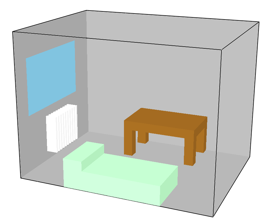
In a room with dimensions of 4 x 3 x 3 m, the radiator is simulated by modeling obstruction with a high surface temperature.
2. Mesh
The computational volume is divided into several meshes.
The meshes increase in definition as their proximity to the radiator increases.
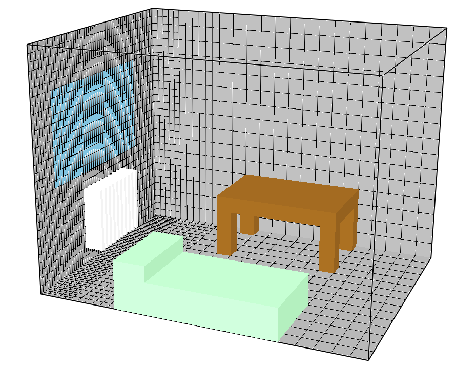
&MESH ID='Grid 01', IJK=15, 15, 15, XB=0, 3, 0, 3, 0, 3/
&MESH ID='Grid 02', IJK=6, 30, 15, XB=3, 3.6, 0, 3, 0, 3/
&MESH ID='Grid 03', IJK=5, 60, 30, XB=4, 3.6, 0, 3, 0, 3/
3. Radiator
The radiator is simulated through different obstructions (OBST) which is assigned a surface (SURF) whose temperature is high. This is done via the TMP_FRONT command.
&OBST XB=3.8, 4, 1.8, 1.85, 0.2,1, COLOR= 'WHITE', SURF_ID='radiator' /
….
….
&OBST XB=3.8, 4, 1.9, 1.95, 0.2,1, COLOR= 'WHITE', SURF_ID='radiator' /
&SURF ID='radiator', TMP_FRONT=70. /
Note for beginners
If you prefer a single, structured learning path that guides you step by step through FDS fundamentals and core concepts, you may want to check the FDS Fundamentals Course.
4. Outputs
As outputs there are slice files that measure the speed and temperature of the air in the environment.
